3 ways how to hide columns in the Excel table

Excel is a unique program, as it has a lot of opportunities, many of which make it possible to significantly simplify work with the tables. This article will talk about one of the features that allows you to hide the columns in the plate. Thanks to her, it will be possible, for example, hide intermediate calculations that will distract attention from the final result. At the moment, several methods are available, each of which will be described in detail below.

Method 1: Protinal Border Shift

This method is as simple as possible and effective. If you consider actions in more detail, then you have to do the following:

1. To begin with, pay attention to the coordinate line, for example, the upper one. If you bring the cursor to the column border, it will change and will look like a black line with two arrows on the sides. This means that you can safely move the border.

So looks like the cursor while changing the border of the column

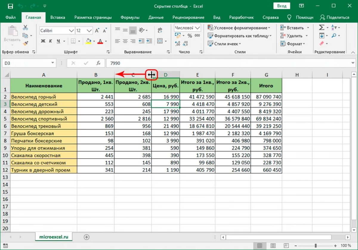
1. If the border is as close as possible to the neighboring border, the column narrows so much that it will not be seen again.

So looks like a column that is hidden

Method 2: Context Menu

This method is the most popular and in demand among all the others. For its implementation, it will be enough to perform a list of the following actions:

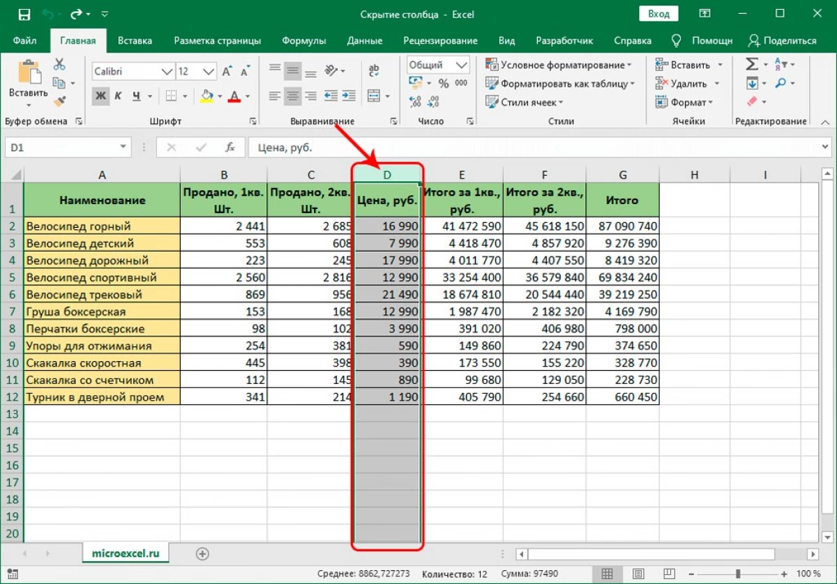
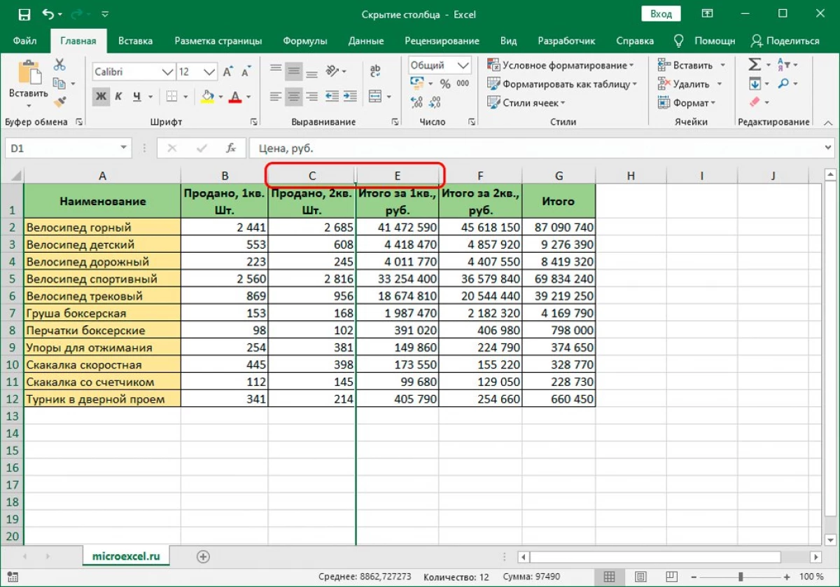
1. To begin with, you must click on the right mouse button on the name of a column.

It is enough to allocate one of the columns

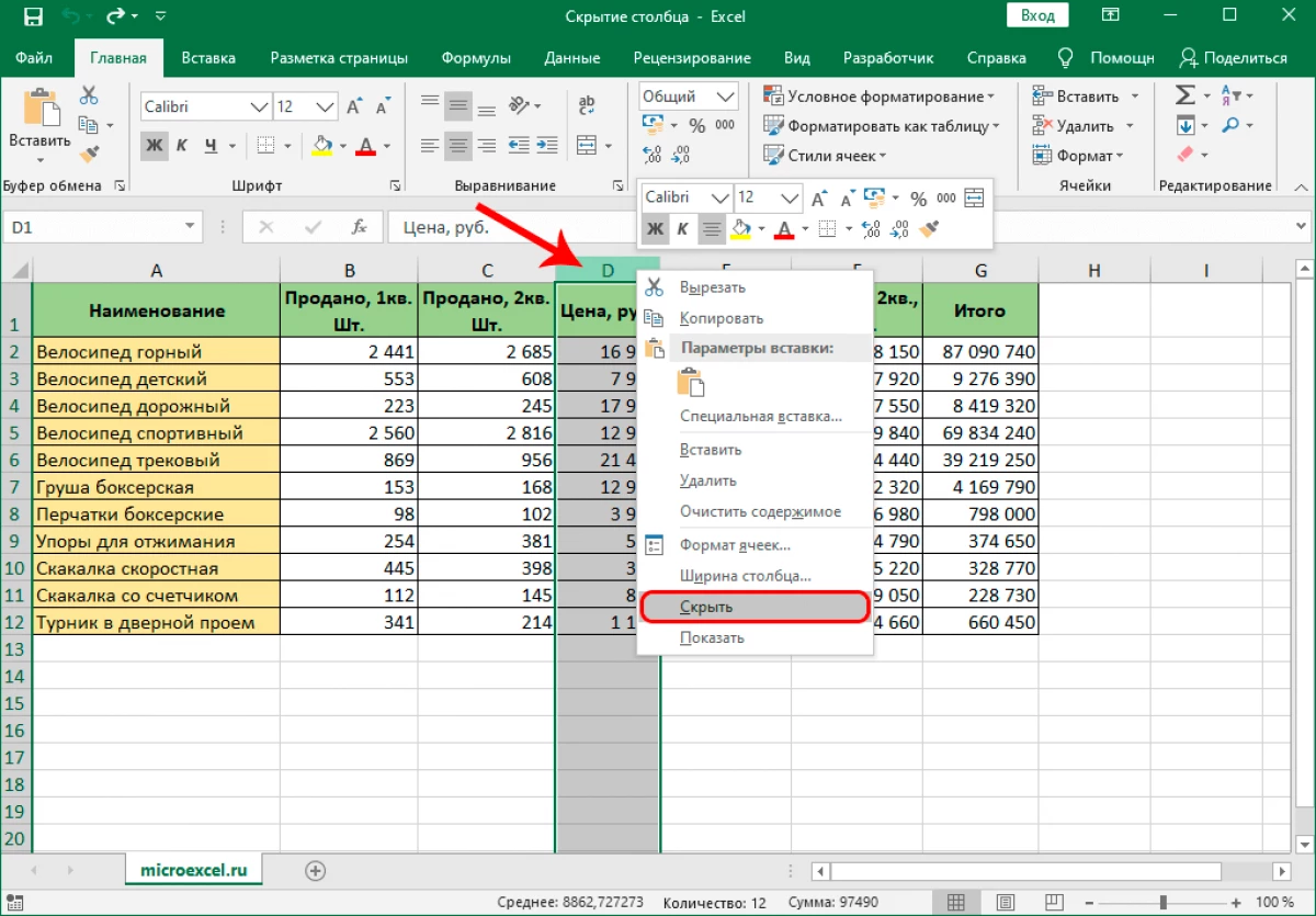
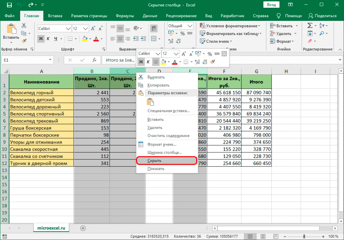
1. A context menu appears, in which it is enough to select "Hide".

Here is the desired item in the context menu

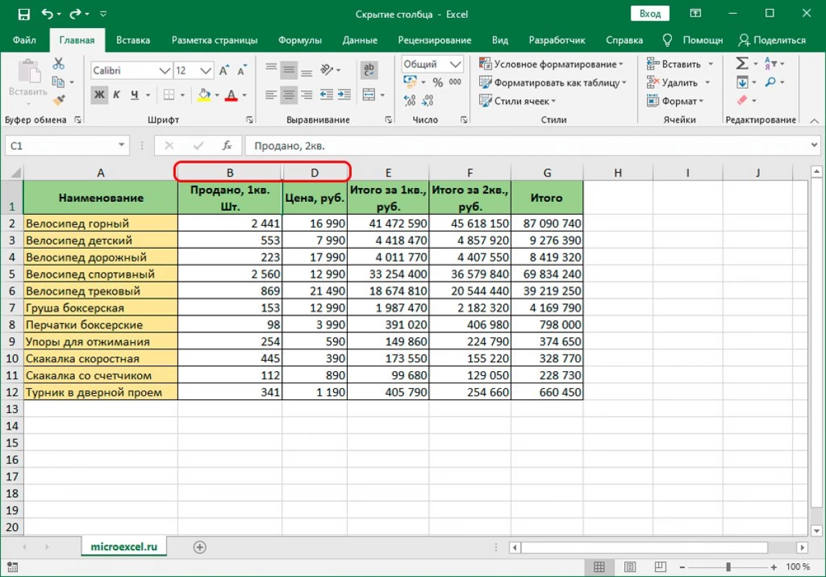
1. After the actions performed, the column will be hidden. It will only be left to try to return it to the original state so that in case of an error it was possible to quickly fix it.

After performing actions, the column will be hidden

1. There is nothing complicated in this, it is enough to choose two columns, between which our main column was hidden. Click on them with the right mouse button and select the "Show" item. After that, the column will appear in the table, and they can be used again.

Thanks to this method, it will be possible to actively use this feature, save time and not suffer with tightening boundaries. This option is the easiest, therefore, is in demand among users. Another interesting feature of this method is that it makes it possible to hide several columns immediately. To do this, it will be enough to perform the following actions:

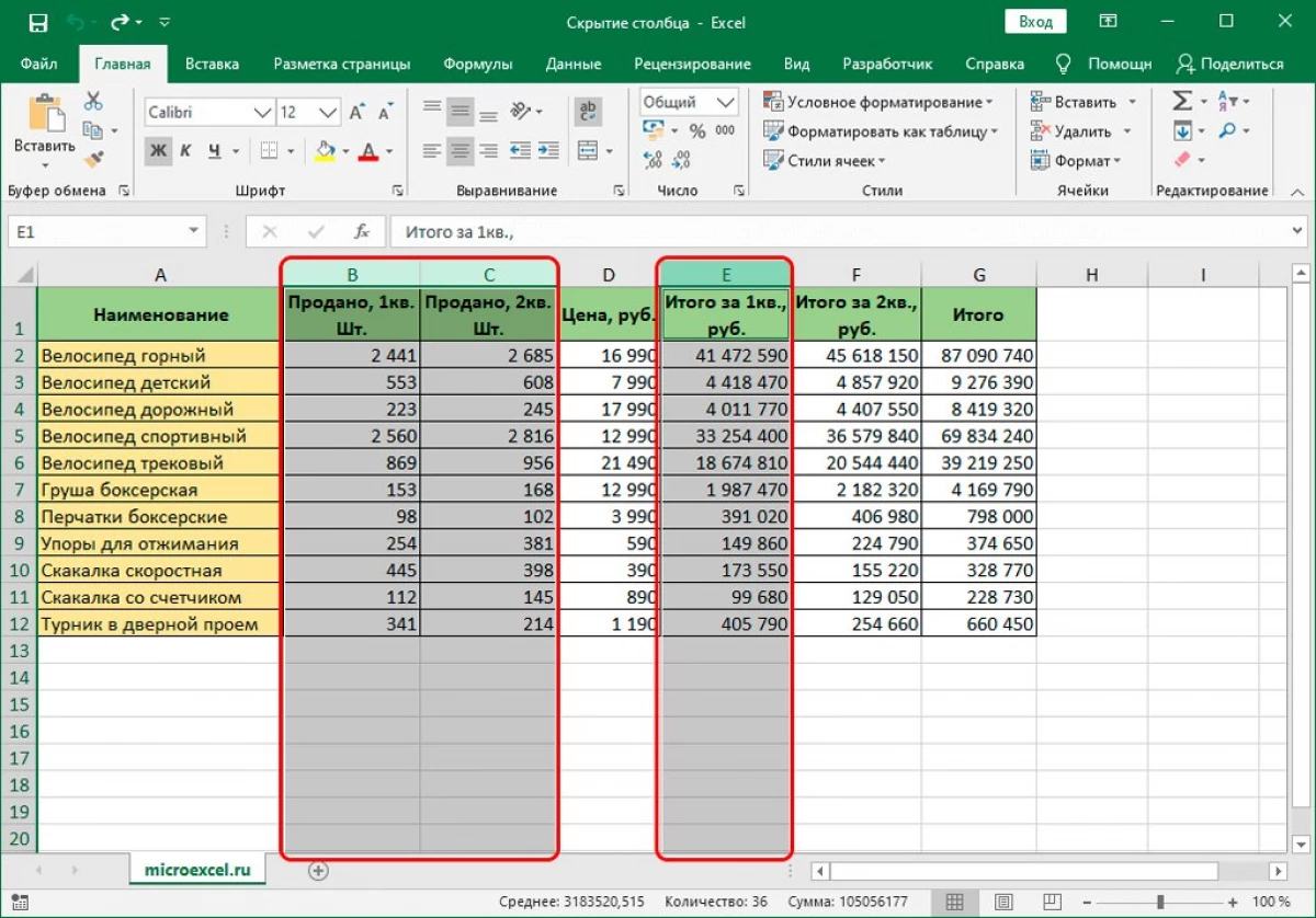
1. To begin with, allocate all columns that need to be hidden. To do this, clamp "Ctrl" and click on the left mouse button onto all columns.

Selection of several columns

1. Next, it is enough to click right-click on the selected column and select "Hide" from the drop-down menu.

The context menu and the function remained unchanged

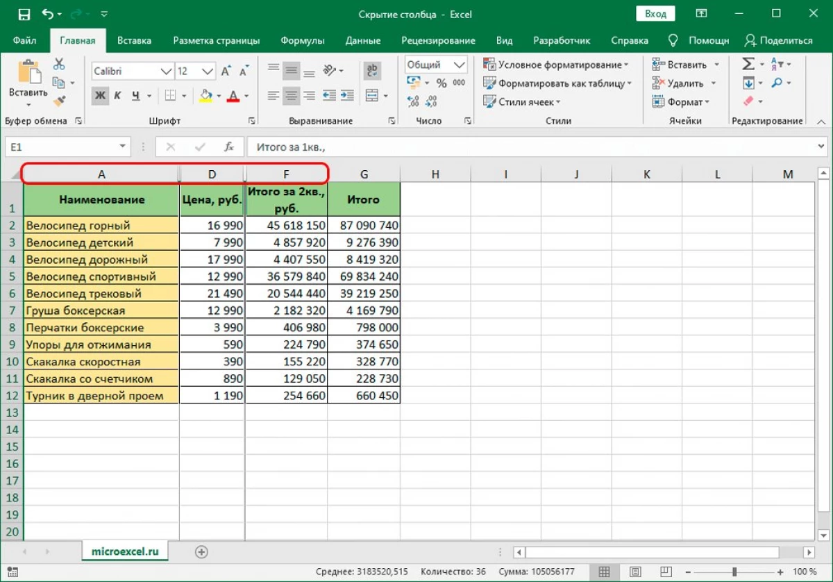
1. After the actions performed, all columns will be hidden.

Visually columns will be hidden similarly to situations when they hid one column

Thanks to such an opportunity, all available columns can be actively hidden, while spending a minimum of time. The main thing is to remember about the order of all actions and try not to hurry to prevent an error.

Method 3: Tools on the ribbon

There is another effective way that will achieve the desired result. This time it is necessary to use the toolbar from above. Step-by-step action is as follows:

1. First of all, select the column cell that you plan to hide.

You can select any cell in the desired column

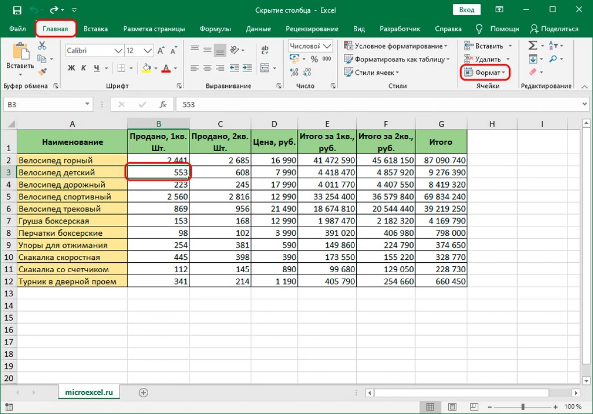
1. Then we turn to the toolbar and use the "Home" section to go to the format item.
2. In the opened menu, you must select the "Hide or Display" item, and then select "Hide Columns".

Step-by-step action

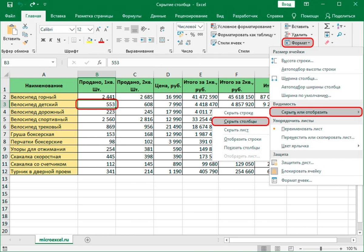
If everything is done correctly, the columns will hide and will no longer load the table. This method extends both to conceal one column and several minutes. As for their reverse scan, the detailed instructions for the implementation of this action were considered above this material, using it, you can easily reveal all previously hidden columns.

Conclusion

Now you have all the necessary knowledge that will continue to actively use the ability to hide extra columns, making the table more convenient for use. Each of the three ways is not complicated and accessible to each user of the Excel table processor - both newcomer and a professional.

Message 3 of the method, how to hide the columns in the Excel table first appeared on information technology.