How to filter data to Excel in color

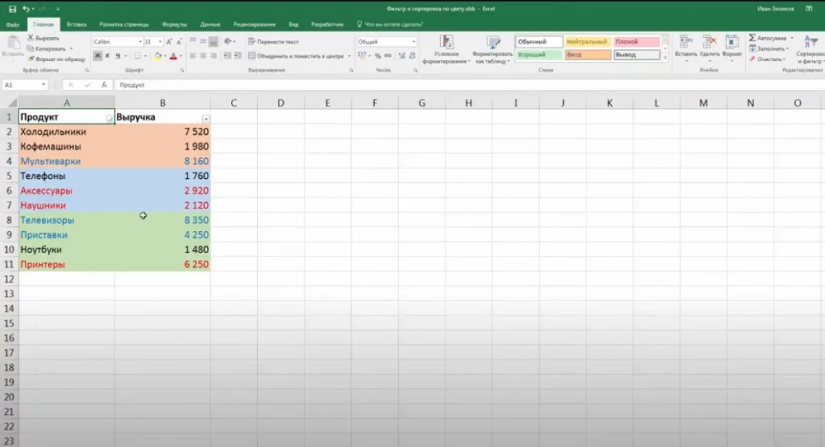
In Microsoft Office Excel, starting in 2007, it has the possibility of sorting and filtering the cells of the table array in color. This function allows faster to navigate in the table, increases its presentability and aesthetics. This article will consider the basic ways to filter information in Excel in color.

Filtering Filtering

Before switching to the consideration of the methods of filtering data in color, it is necessary to analyze the advantages that this procedure gives:

• Structuring and streamlining information, which allows you to select the desired fragment of the plate and quickly find it in a large range of cells.
• Cell-highlighted cells with important information can be analyzed in the future.
• Filtering in color allocates information that satisfy the specified criteria.

How to filter out the color data using the built-in Excel options

The color filtering algorithm in the Excel table array is divided into the following steps:

1. Select the desired range of cells with the left key of the manipulator and move to the "Home" tab located in the top of the program toolbar.
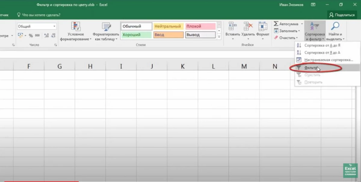
2. In the area that appears in the subsection, editing you need to find the "Sort and Filter" button and deploy it by clicking on the arrow below.

Options for sorting and filtering tabular data in Excel

1. In the displayed menu, click on the filter line.

In the selection window, click on the "Filter" button

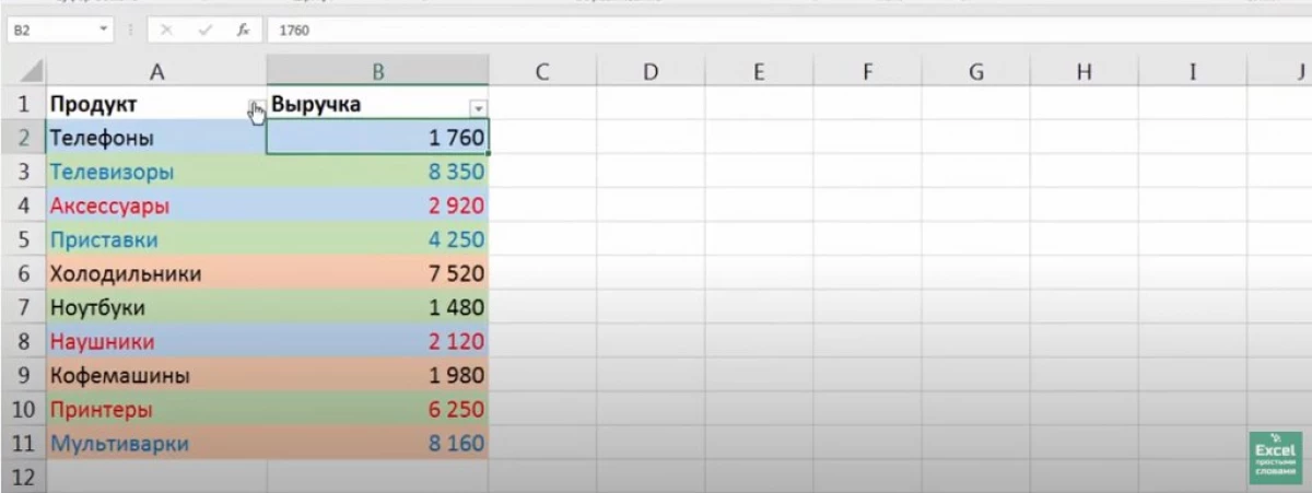
1. When the filter is added, then small arrows will appear in the table columns. At this stage, by any of the arrows, the user needs to click LKM.

Arrogo appeared in table column headers after adding a filter

1. After pressing the arrow in the name of the column, a similar menu is displayed, in which you need to click on the line filter string. An additional tab with two available features will be revealed: "Cell Flower Filter" and "Font Color Filter".

Filtration options in Excel. Here you can choose any color to be located on top of the table

1. In the "Cell Color Filter" section, select the shade for which you need to filter the source table by pressing the LKM on it.
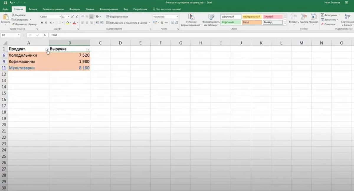
2. Check the result. After spending the above manipulations, only cells with the previously specified color will remain in the table. The remaining elements will disappear, and the plate is reduced.

The appearance of the plate transformed after filtering data in it

Filter data in an Excel array can be manually, deleting strings and columns with unnecessary colors. However, the user will have to spend extra time for this process.

If you select the desired shade in the Font Color Filter section, only lines will remain in the table, the font text in which is registered with the selected color.

How to sort data on multiple colors in Excel

With sorting in colors in Excel, there are usually no problems. It is performed in the same way:

1. By analogy with the previous point, add a filter to a table array.
2. Click on the arrow that appeared in the column name, and in the drop-down menu select "Sort by Color".

Selecting color sorting

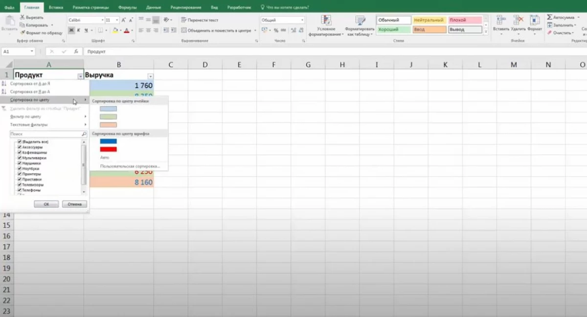
1. Specify the desired type of sorting, for example, select the desired shade in the "Cell Column" column.
2. After completing the previous manipulations, the table lines with the previously selected tint will be located in the first place of the array in order. You can also sort the remaining colors.

The final result of sorting cells in color in the table array

How to filter information in the table by color using the user function

To select a filter in Microsoft Office Excel to display several colors at once in the table, you need to create additional parameters with a shade of fill. According to the created shade, the data in the future will be filtered. The user function in Excel is created according to the following instructions:

1. Go to the "Developer" section, which is located on top of the main menu of the program.
2. In the currently opened tab, click on the "Visual Basic" button.
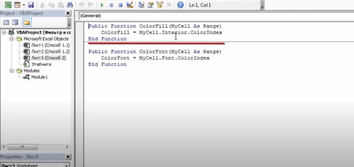
3. The built-in program will open, in which you will need to create a new module and register the code.

Program code with two functions. The first determines the color of the fill of the element, and the second is responsible for the color inside the cell

To apply the created function, you need:

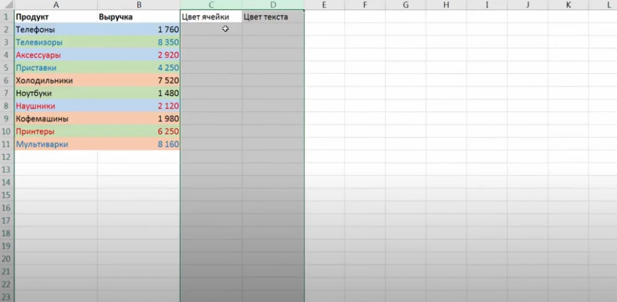
1. Return to the Excel working sheet and create two new columns next to the source table. They can be called "Cell Color" and "Text Color", respectively.

Created auxiliary columns

1. In the first column, write the formula "= Colorfill ()". The brackets indicate the argument. You need to click on the cell with any color in the plate.

Formula in Column "Cell Color"

1. In the second column, specify the same argument, but only with the "= ColorFont ()" function.

Formula in column "Text color"

1. Stretch the resulting values ​​to the end of the table, extinguishing the formula for the entire range. The data obtained is responsible for the color of each cell in the table.

The resulting data after stretching the formula

1. Add a filter to a table array according to the above scheme. The data will be sorted by color.

Conclusion

Thus, in MS Excel, you can quickly filter the source table array in the color of the cells in various methods. The main methods of filtering and sorting, which are recommended to use when performing the task, were considered above.

Message How to filter out data in Excel in color appeared first to information technology.