How to remove the filter in Excel

Data filtering in Excel is necessary to facilitate working with tables and large amounts of information. So, for example, a significant part can be hidden from the user, and when activating the filter, display the information that is currently necessary. In some cases, when the table was created incorrectly, or for the reasons of the inexperience of the user, there is a need to remove the filter in separate columns or on the sheet completely. How exactly it is done, we will analyze in the article.

Examples of table creation

Before you start removing the filter, first consider options for its inclusion in the Excel table:

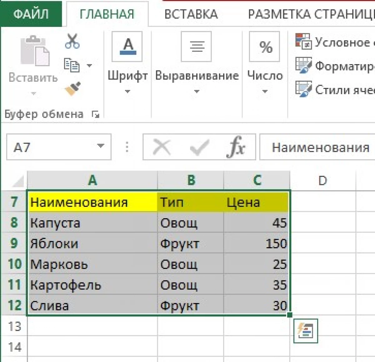
• Manual data entry. Fill the rows and columns with the necessary information. After that, select the addressing of the table location, including headlines. Go to the "Data" tab at the top of the tools. We find a "filter" (it is displayed in the form of a funnel) and click on it by the LKM. The filter is activated in the upper headers.

one

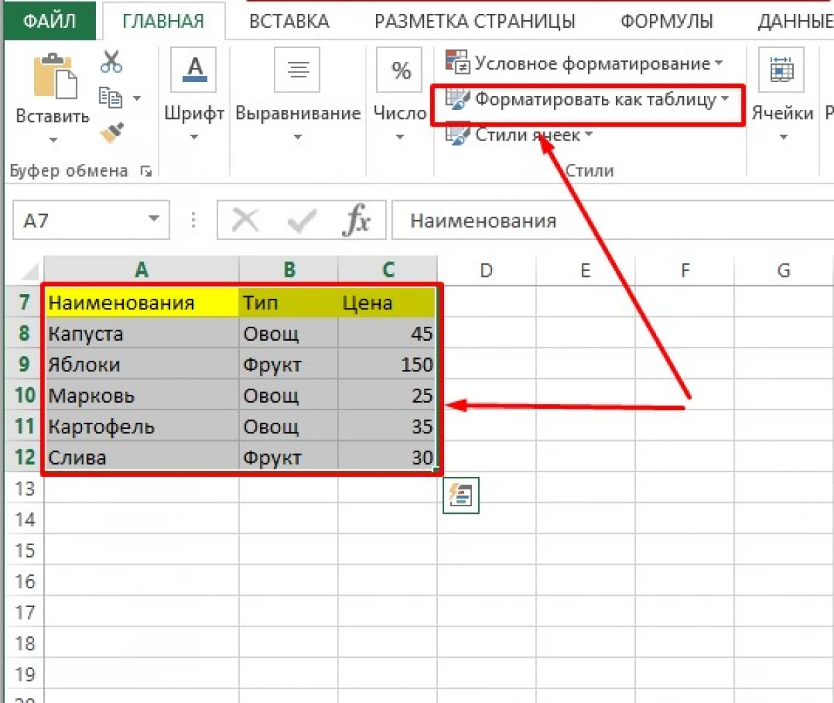
• Automatic filtering on. In this case, the table is also pre-filled, after which in the "Styles" tab, it is found to activate the "Filter As Table" string. There should be automatic filters in the subtitles of the table.

2.

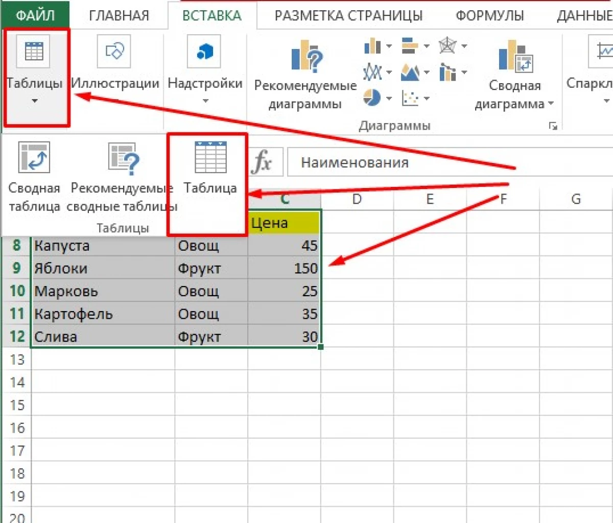
In the second case, you need to go to the "Insert" tab and finding the Table Tool, click on it with the LKM and from the following three options to select "Table".

3.

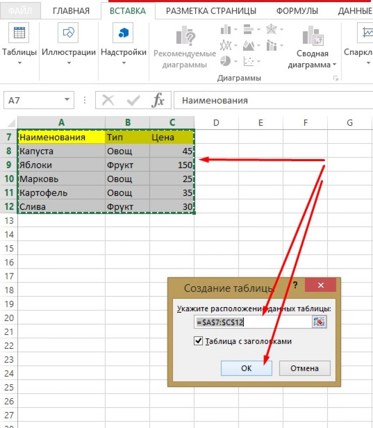
The following interface window that opens, the addressing of the created table is displayed. It remains only to confirm it, and the filters in the subtitles are automatically turned on.

four

Examples with filter in Excel

Leave to consider the same sample table created earlier on three columns.

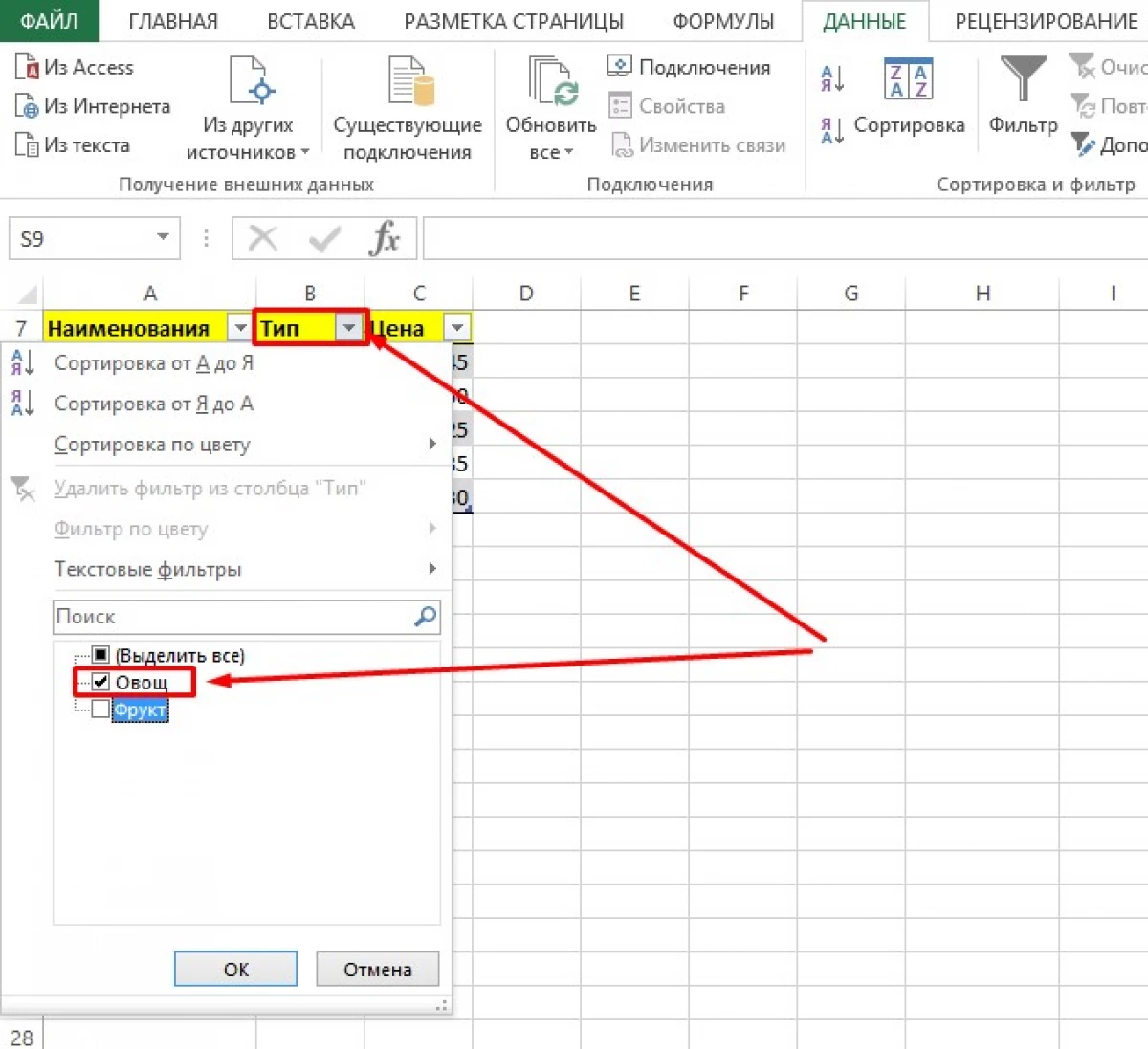
• Select a column where you need to adjust. By clicking on the arrow in the upper cell, you can see a list. To remove one of the values ​​or items, you must remove the tick on the contrary.
• For example, we need only vegetables in the table. In the window that opens, remove the tick with the "fruit", and leave the vegetables active. Agree by clicking on the "OK" button.

five

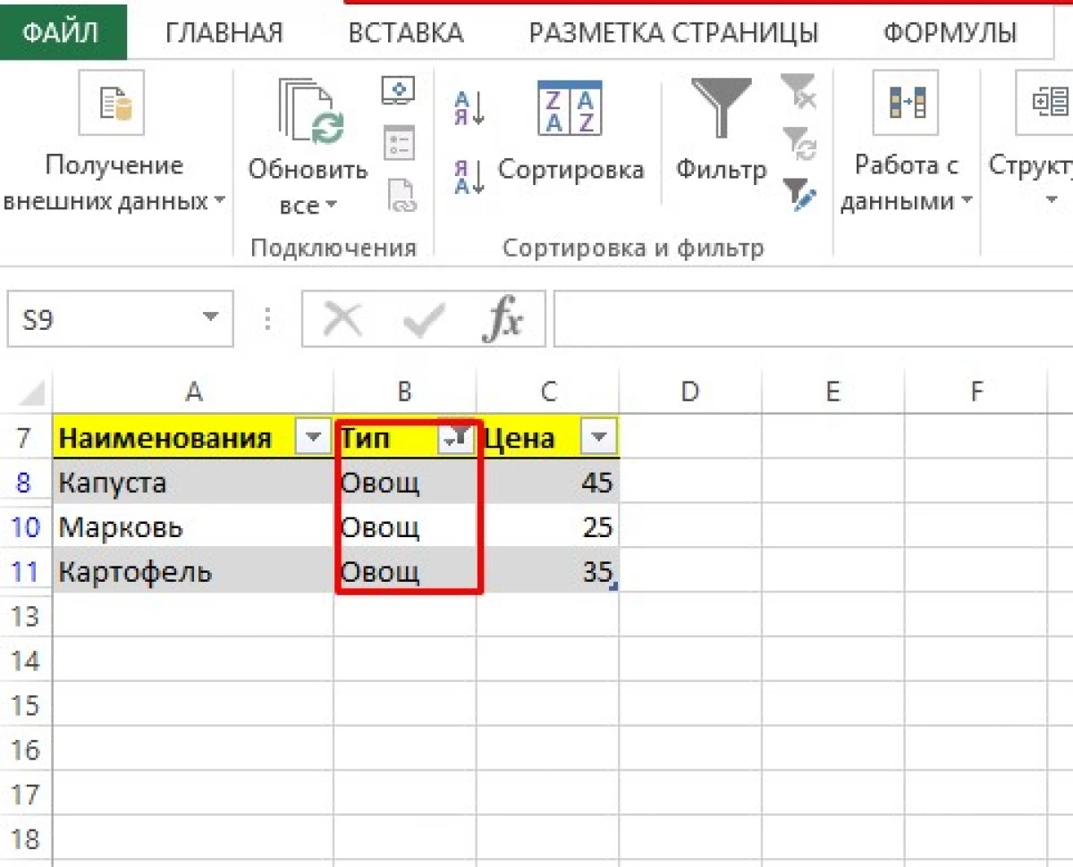
• After activating the list will look like this:

6.

Consider another example of filter operation:

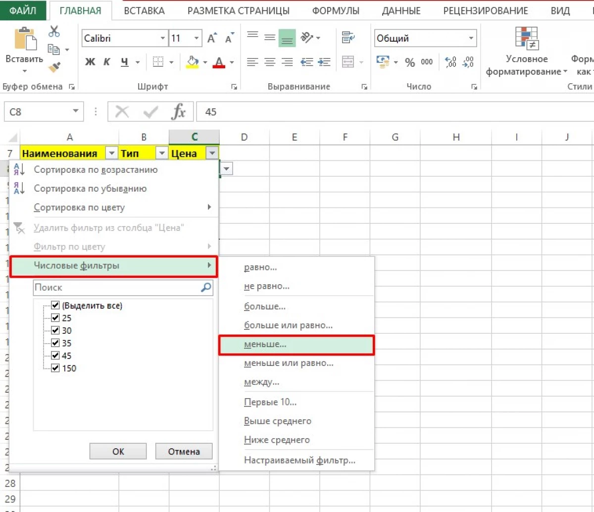
• The table is divided into three columns, and the last prices for each type of product are presented. It needs to be adjusted. Suppose we need to filter products whose price is lower than the value "45".
• Click on the filtering icon in the cell selected by us. Since the column is filled with numeric values, then in the window you can see that the "Numeric filters" string is in an active condition.
• Having a cursor on it, open a new tab with different features of the digital table filtering. In it, choose the value "less".

7.

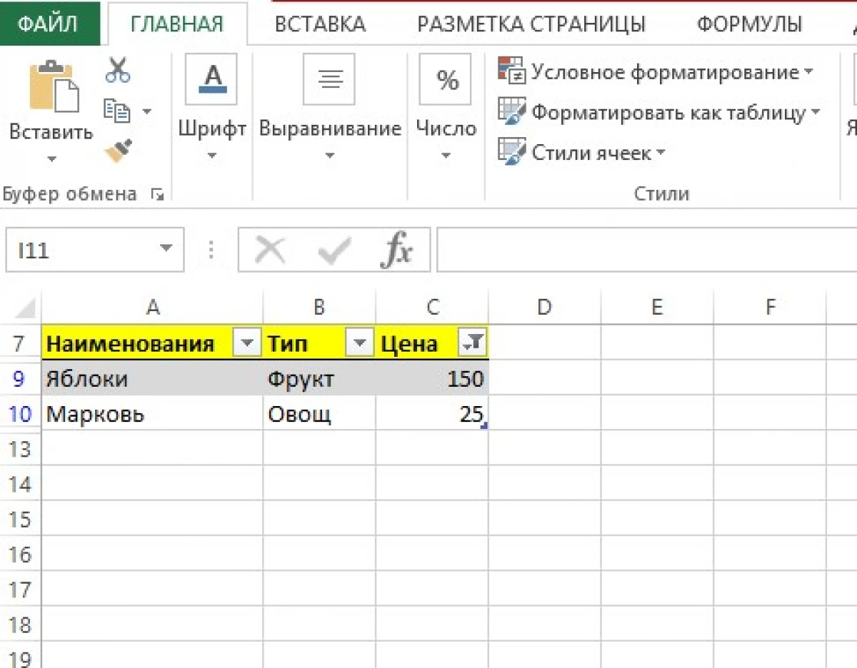
• Then enter the number "45" or choose by opening a list of numbers in a user autofilter.

Also, with the help of this function, prices are filtered in a specific digital range. To do this, you need to activate the "or" button in the user autofilter. Then at the top set the value "less", and below "more". In the interface strings on the right, the required parameters of the price range are set to leave. For example, less than 30 and more than 45. As a result, the table will retain numeric values ​​25 and 150.

eight

The possibilities of filtering information data are actually extensive. In addition to the examples, it is possible to adjust the data on the color of the cells, according to the first letters of names and other values. Now, when we conducted a general familiarization with the methods of creating filters and the principles of working with them, go to removal methods.

Remove column filter

1. First, we find a saved file with a table on your computer and a double click LKM open it in Excel. On a sheet with a table, you can see that the filter is in an active condition in the price column.

nine

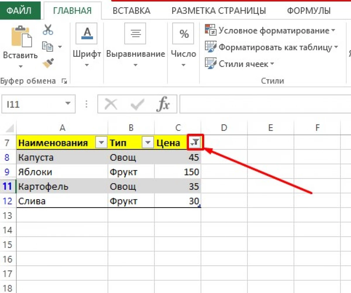
1. Click on the arrow icon down.
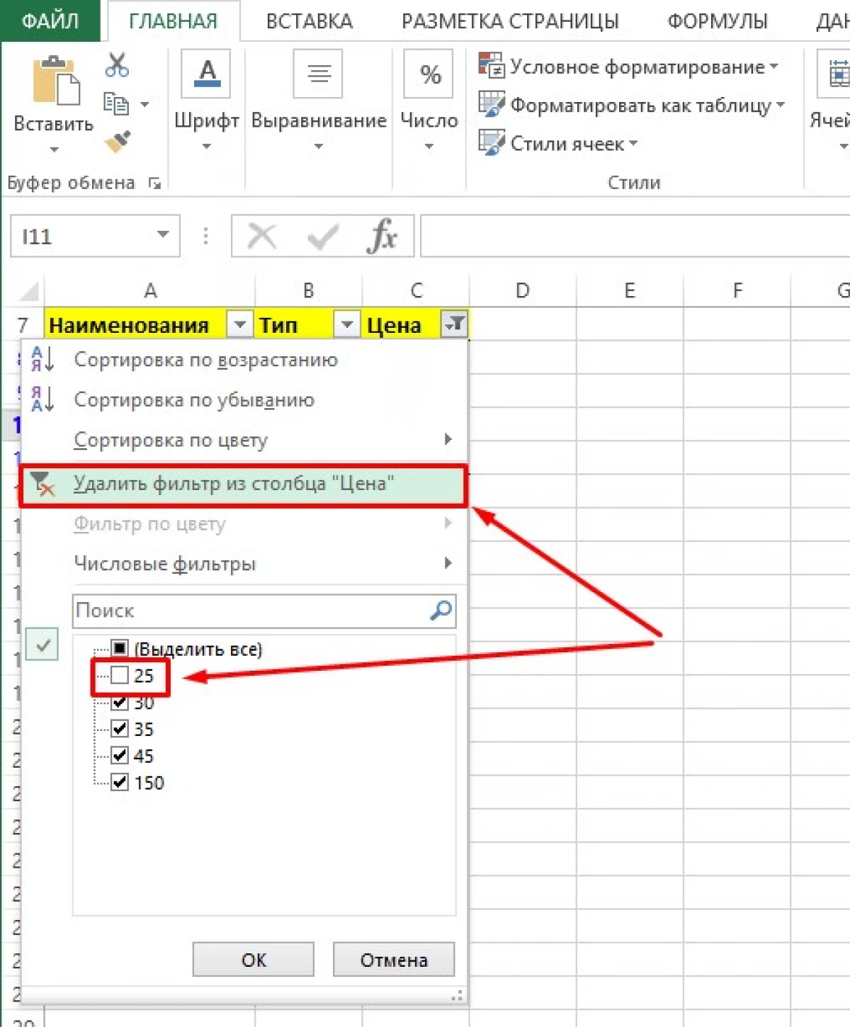
2. In the dialog box that opens, you can see that the check mark opposite the numbers "25" is removed. If active filtering was removed only in one place, then the easiest way to install the label back and click on the "OK" button.
3. Otherwise, it is necessary to turn off the filter. To do this, in the same window you need to find the string "Delete a filter from the column" ... "and click on it LKM. There will be automatic shutdown, and all previously entered data will be displayed in full.

10

Removing a filter from a whole sheet

Sometimes situations may occur when the need to remove the filter in the entire table appears. To do this, you will need to perform the following actions:

1. Open the file with the saved data in Excel.
2. Find one column or several where the filter is activated. In this case, this is the "name" column.

eleven

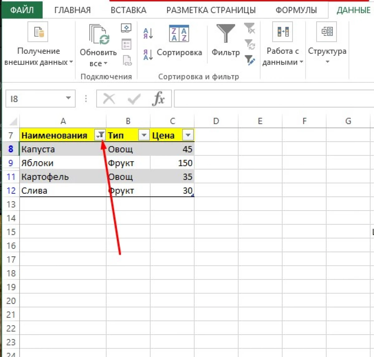
1. Click on any place in the table or highlight it completely.
2. At the top, find the "data" and activate their LKM.

12

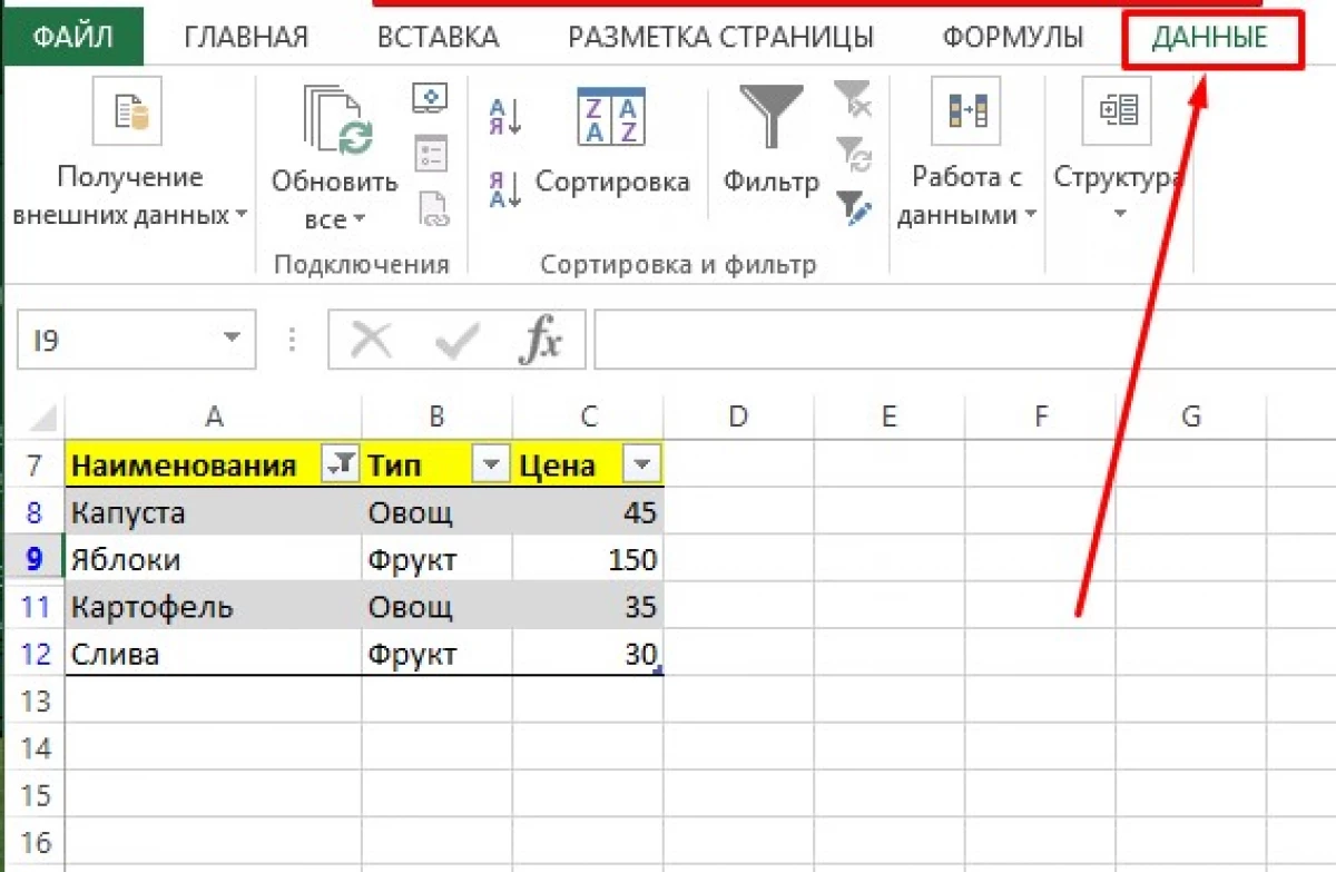
1. Lay "Filter". Opposite the column is three symbols in the form of a funnel with different modes. Click on the functional button "Clear" with the displayed funnel and red crosshair.
2. Next will turn off active filters throughout the table.

Conclusion

Filtering elements and values ​​in the table greatly facilitates work in Excel, but unfortunately, the person is inclined to make mistakes. In this case, the Multifunctional Excel program comes to the rescue, which will help sort the data and remove unnecessary filters entered earlier with the preservation of the source data. This feature is especially useful when filling in large tables.

Message How to remove the filter in Excel appeared first to information technology.