How to add a legend in the Excel 2010 chart

In Microsoft Office Excel, you can quickly build a diagram along the table array drawn up to reflect its main characteristics. The diagram is made to add a legend to characterize the information depicted on it, give them the name. This article discovers the methods of adding legend to the chart in Excel 2010.

How to build a chart in Excel on the table

First, it is necessary to understand how the diagram is built in the program under consideration. The process of its construction is conditionally divided into the following steps:

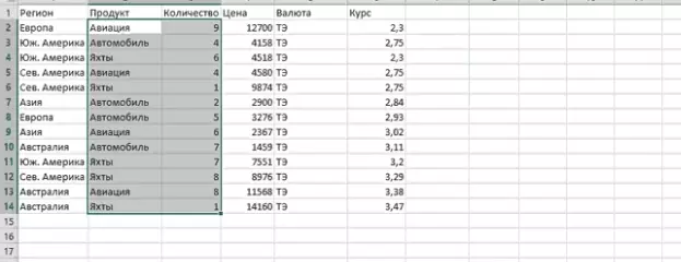
1. In the source table, select the desired range of cells, the columns for which the dependency must be displayed.

Select the required range of cells in the table to build a chart

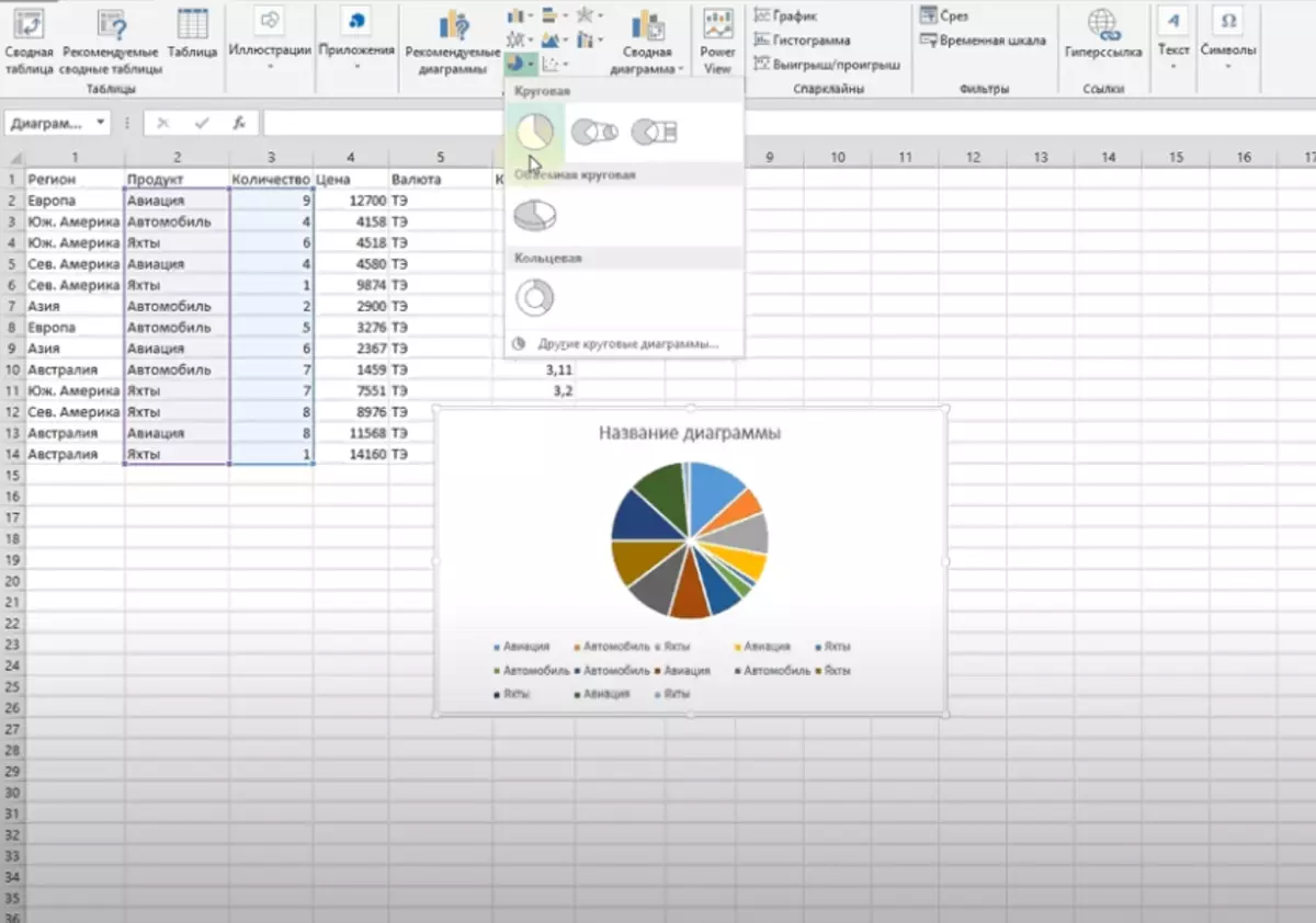
1. Go to the "Insert" tab in the upper graph of the main menu of the program.
2. In the "diagram" block, click on one of the variants of the graphic representation of the array. For example, you can choose a circular or bar chart.

Actions to build a chart in Excel 2010

1. After completing the previous action, a window with a built diagram should appear next to the original name plate on the Excel. It will reflect the dependence between the values ​​deemed in the array. So the user can clearly appreciate the differences in the values, analyze the schedule and conclude on it.

How to add a legend to a chart in Excel 2010 in a standard way

This is the easiest method of adding a legend that does not take the user a lot of time to implement. The essence of the method is to do the following steps:

1. Build a diagram on the above scheme.
2. Left key manipulator Press the green cross icon in the toolbar to the right of the graph.
3. In the above options window that opens next to the legend string, put a tick to activate the function.

Staging a tick next to the line "Legend" for its display on the built schedule

1. Analyze the diagram. It should add signatures of elements from the source table array.
2. If necessary, you can change the location of the schedule. To do this, click the LKM on the legend and choose another option of its location. For example, "on the left", "bottom", "top", "right" or "on top of the left".

Changing the location of the diagram in the block on the right window

How to change the text of the legend in the chart in Excel 2010

Sappings of the legend, if desired, can be changed by setting the appropriate font and size. You can do this operation according to the following instructions:

1. Build a diagram and add a legend to it on the algorithm discussed above.
2. Amend the size, text font in the source table array, in the cells on which the schedule itself is built. When formatting text in the columns of the table, the text in the legend of the chart will automatically change.
3. Check the result.

How to fill in a chart

In addition to the legend, there are several more data that can be reflected on the built schedule. For example, its name. To name the built object, it is necessary to act as follows:

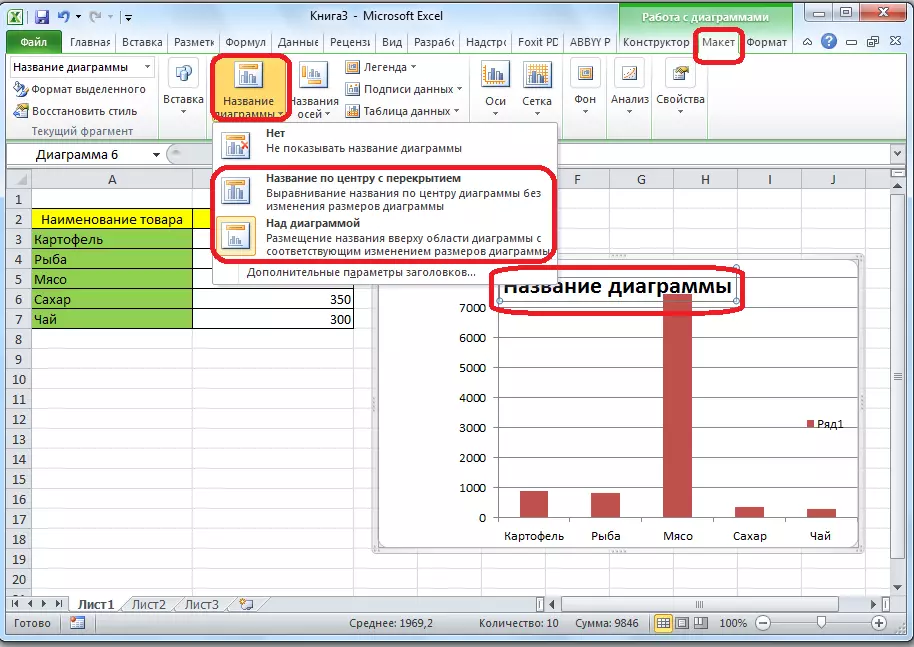
1. Build a diagram on the source plate and move to the "Layout" tab on top of the main program menu.
2. The area of ​​work with diagrams will open, in which several parameters are available to change. In this situation, the user needs to click on the "Diagram Title" button.
3. In the expanded list of options, select the type of location type. It can be placed in the center with overlapping, or above the schedule.

Adding titles to a chart in Microsoft Office Excel

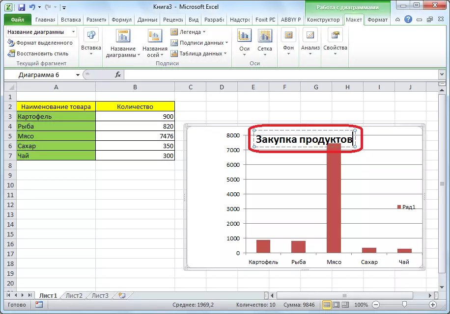
1. After executing previous manipulations, the inscription "Diagram" appears on the built graph. Its user will be able to change, prescribing manually from the computer keyboard any other combination of words suitable in meaning to the source table array.

Change added to the name of the name

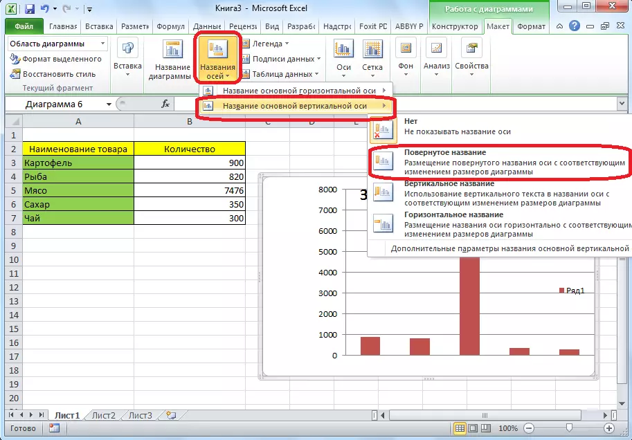
1. It is also important to sign the axis on the schedule. They subscribe in the same way. In the work block with charts, you will need to click on the "axis name" button. In the unfolded list, select one of the axes: either vertical or horizontal. Next, make the appropriate change for the selected option.

Signing axes in the chart

Alternative method for changing the legend chart in Excel

You can edit the text of signatures on the schedule using the tool built into the program. To do this, you need to do a few simple steps on the algorithm:

1. Right-key manipulator click on the desired word legend in the constructed chart.
2. In the contextual window window, click on the "Filters" line. After that, the window of custom filters opens.
3. Click on the "Select Data" button, located at the bottom of the window.

Legend properties window in Excel

1. In the new menu "Select data sources", you must click on the "Change" in the "Legend" block.
2. In the next window in the "Row name" field, you will register a different name for the previously selected element and click on "OK".

Writing a new name for graph elements

1. Check the result.

Conclusion

Thus, the construction of a legend in Microsoft Office Excel 2010 is divided into several stages, each of which needs a detailed study. If you wish, the information on the chart can quickly edit. Above the basic rules of work with charts in Excel were described.

Message How to add a legend in the Excel 2010 chart appeared first to information technology.