Excel Sensitivity Analysis (Data Table Sample)

Finance processes are always interrelated - one factor depends on the other and changes with it. Tracking these changes and understand what to expect in the future is possible using Excel functions and tabular methods.

Obtaining multiple results using a data table

The capabilities of the data tables are elements of the "what if" analysis is often carried out through Microsoft Excel. This is the second name of the sensitivity analysis.

General

The data table is the type of cell range, with which you can solve the problems arising by changing the values ​​in some cells. It is made when it is necessary to monitor changes in the components of the formula and receive updates of the results, according to these changes. Find out how to apply data tablets in studies, and which species they are.

Basic information about data tables

There are two types of data tables, they differ in the number of components. Make a table is needed with orientation by the number of values ​​that need to be checked with it.

Statistics specialists apply a table with one variable when there is only one variable in one or several expressions, which may affect the change in their result. For example, it is often used in a bundle with the PL function. The formula is designed to calculate the amount of regular pay and takes into account the interest rate set in the contract. With such calculations, the variables are recorded in one column, and the results of calculations to another. An example of data plate with 1 variable:

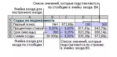
one

Next, consider signs with 2 variables. They apply in cases where two factors affect the change in any indicator. Two variables may be in another table associated with a loan - with its help you can identify the optimal payment period and the amount of the monthly payment. This calculation also needs to use the PPT function. An example plate with 2 variables:

2 Creating a data table with one variable

Consider the analysis method on the example of a small bookstore, where only 100 books are available. Some of them can be sold more expensive ($ 50), the rest will cost buyers cheaper ($ 20). The total income from the sale of all goods is designed - the owner decided that in a high price of 60% of books. It is necessary to find out how revenue will grow if you increase the price of a larger volume of goods - 70% and so on.

1. Choose a free cell distance from the edge of the sheet and write the formula in it: = the cell of the total revenue. For example, if the income is recorded in the C14 cell (a random designation is indicated), it is necessary to write like this: = C14.
2. We write down the amount of goods in the column to the left of this cell - not under it, it is very important.
3. We allocate the range of cells where the interest column is located and a link to the total income.

3.

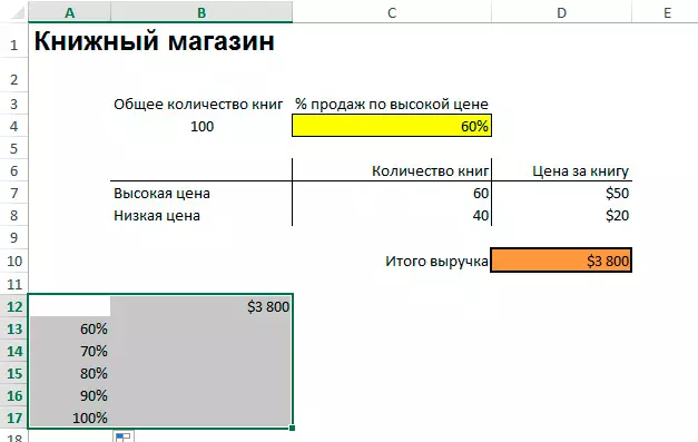
1. We find on the "Data" tab of the "Analysis" What if "" and click on it - in the menu that opens, you need to select the "Data Table" option.

four

1. A small window will open, where you need to specify a cell with a percentage of the books originally sold at a high price in the column "to substitute values ​​on the lines in ...". This step is done to make recalculation of general revenue, taking into account the increasing percentage.

five

After pressing the "OK" button in the window where data was entered to compile the table, the results of the calculations will appear in the rows.

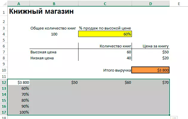
Adding a formula to a data table with one variable

From the table that helped calculate the action with only one variable, you can make a complicated analysis tool by adding an additional formula. It must be entered near the already existing formula - for example, if the table is focused on rows, enter the expression into the cell to the right of the already existing one. When the orientation is installed on columns, write down a new formula under the old. Next should be acting according to the algorithm:

1. We again highlight the range of cells, but now it should include a new formula.
2. Open the "What if" analysis menu and select "Data Table".
3. Add a new formula to the corresponding field on line or by columns, depending on the orientation of the plate.

Creating a data table with two variables

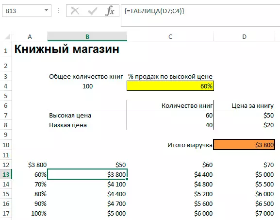
The beginning of the preparation of such a table is slightly different - you need to place a link to the overall revenue above the percent values. Next, we perform these steps:

1. Record options for the price of one line with reference to income - each price is one cell.
2. Select the range of cells.

6.

1. Open the data table window, as when drawing up a single variable - via the Data tab on the toolbar.
2. Substitute in the Count "To substitute values ​​on columns in ..." cell with an initial high price.
3. Add to the column "To substitute values ​​on strings in ..." cell with an initial interest in sales of expensive books and click "OK".

As a result, the entire plate is filled with the amounts of possible income with different terms of sale of goods.

7 Acceleration of calculations for sheets containing data tables

If quick calculations are required in the data plate that do not run the entire book recalculation, you can perform several actions to speed up the process.

1. Open the parameters window, select the clause "Formula" in the menu on the right.
2. Select the item "Automatically, except for data tables" in the "Calculations in the book" section.

eight

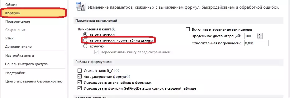
1. Perform the recalculation of the results in the plate manually. For this you need to highlight the formulas and press the F key

Other tools for performing sensitivity analysis

The program has other tools to help perform sensitivity analysis. They automate some actions that otherwise would have to be done manually.

1. The "Selection of the parameter" function is suitable if the desired result is known, and it is required to find out the input value of the variable to obtain such a result.
2. "Solution Search" is an add-in to solve problems. It is necessary to establish limitations and indicate them, after which the system will find the answer. The solution is determined by changing the values.
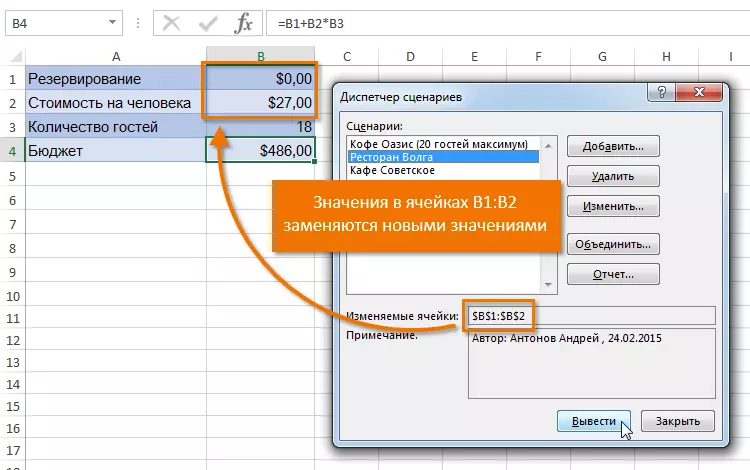
3. Sensitivity analysis can be carried out using the script manager. This tool is in the "What if" analysis menu on the Data tab. It substitutes the values ​​into several cells - the amount can reach 32. The dispatcher compares these values, and the user does not have to change them manually. An example of applying scripting manager:

nine

Analysis of the sensitivity of the investment project in Excel

Method for analyzing sensitivity in the field of investment

When analyzing "What if" uses the bust - manual or automatic. Known range of values, and they are in turn substituted in the formula. As a result, a set of values ​​is obtained. Of these, choose a suitable figure. Consider four indicators for which the analysis of the sensitivity in the field of finance:

1. Pure present value - is calculated by subtracting the size of the investment from the amount of income.
2. The internal rate of profitability / profits - indicates which profit is required from investment for the year.
3. The payback ratio is the ratio of all profits to the initial investment.
4. Discounted profit index - indicates the effectiveness of the investment.

Formula

The sensitivity of the attachment can be calculated using this formula: change the output parameter in% / change in the input parameter in%.

The output and input parameter may be the values ​​described earlier.

1. It is necessary to know the result under standard conditions.
2. We replace one of the variables and follow the results of the result.
3. Calculate the percentage change in both parameters relative to the established conditions.
4. We insert the percentages obtained into the formula and determine the sensitivity.

An example of an analysis of the sensitivity of the investment project in Excel

For a better understanding of the analysis techniques, an example is required. Let us analyze the project with such well-known data:

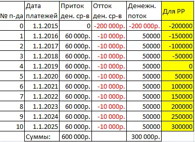
10

1. Fill the table to analyze the project on it.

eleven

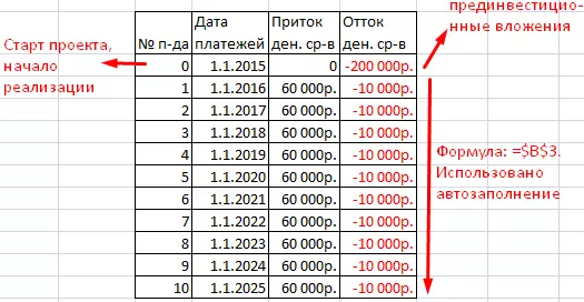
1. Calculate the cash flow using the displacement function. At the initial stage, the flow is equal to investments. Next we use the formula: = If (displacement (number; 1;) = 2; sums (inflow 1: outflow 1); sums (inflow 1: outflow 1) + $ B $ 5) The designations of cells in the formula may be different, it depends on Placement table. At the end, the value from the initial data is added - the liquidation value.

12

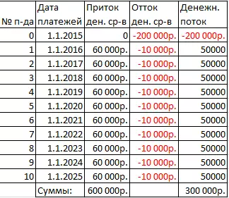
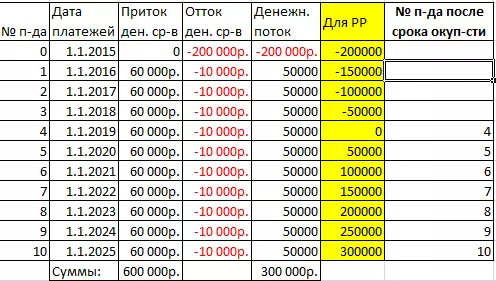
1. We define the deadline for which the project will pay off. For the initial period, we use this formula: = silent (G7: G17; "0; first d.potok; 0). The project is at the break-even point for 4 years.

13

1. Create a column for numbers of those periods when the project pays off.

fourteen

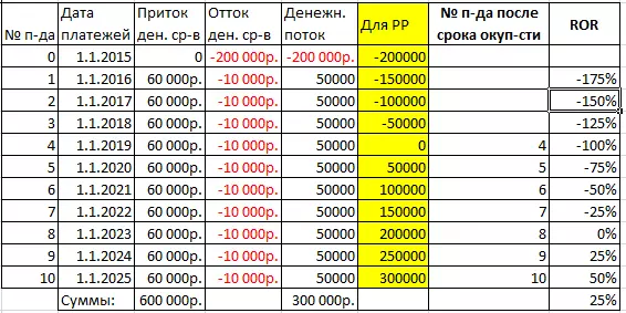
1. Calculate the profitability of investments. It is necessary to create an expression, where the profit in a particular period of time is divided into initial investments.

fifteen

1. Determine the discounting coefficient for this formula: = 1 / (1 + disc.%) ^ Number.

sixteen

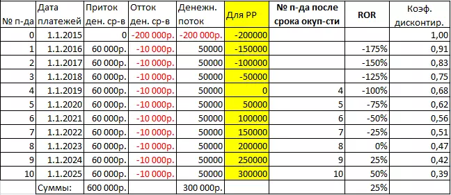
1. Calculate the present value by multiplication - the cash flow is multiplied by the discount rate.

17.

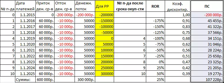
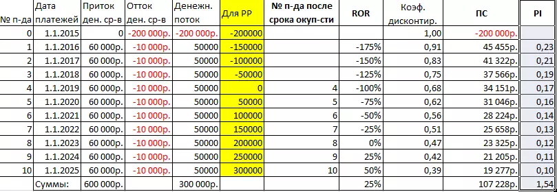
1. Calculate PI (profitability index). The given value in the segment of time is divided into attachments at the beginning of the project development.

eighteen

1. We define the internal rate of profits using the function of the EMD: = FMR (cash flow range).

Analysis of investment sensitivity using the data table

For analysis of projects in the field of investment, other methods are better suited than the data table. Many users have confusion when drawing up the formula. To find out the dependence of one factor from changes in others, you need to select the correct calculation cells and to read the data.

Factor and dispersion analysis in Excel with automation of calculations

Dispersion analysis in Excel

The purpose of such an analysis is to divide the variability of the magnitude of three components:

1. Variability as a result of the influence of other values.
2. Changes due to the relationship of values ​​affecting it.
3. Random changes.

Perform a dispersion analysis through an Excel add-on "Data Analysis". If it is not enabled, it can be connected in parameters.

The starting table must comply with the two rules: each value accounts for one column, and the data in it is arranged in ascending or descending. It is necessary to test the impact of the level of education on behavior in conflict.

nineteen

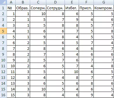
1. We find the "Data" tab "Data" tool and open its window. The list needs to select single-factor dispersion analysis.

twenty

1. Fill out the rows of the dialog box. The inlet interval is all cells without taking into account the caps and numbers. We group on columns. Tell results on a new sheet.

21.

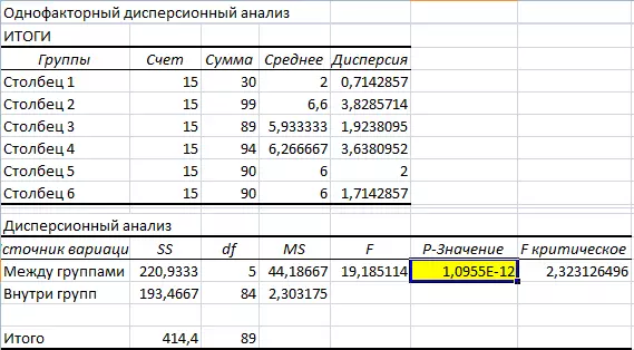
Since the value in the yellow cell is greater than the unit, we can assume the assumption of incorrect - there is no relationship between education and behavior in the conflict.

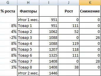
Factor analysis in Excel: Example

We analyze the relationship between data in the field of sales - it is necessary to identify popular and unpopular goods. Initial information:

22.

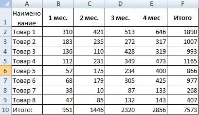
1. It is necessary to find out which goods the demand for the second month has grown over the second month. We make a new table to determine the growth and reduction of demand. The growth is calculated according to this formula: = if (((demand 2-demand 1)> 0; demand 2 - demand 1; 0). The formula of the decline: = if (growth = 0; demand is 1- demand 2; 0).

23.

1. Calculate the growth in demand for goods in percent: = if (growth / total 2 = 0; reduction / total 2; height / total 2).

24.

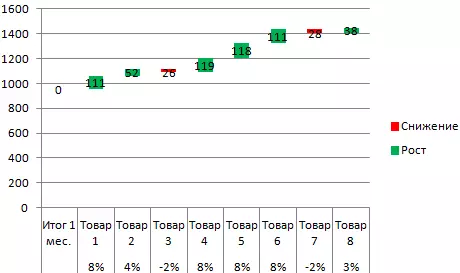
1. We will make a chart for clarity - allocate the range of cells and create a histogram through the "Insert" tab. In the settings you need to remove the fill, it can be done through the "Data format format" tool.

25 Two-factor dispersion analysis in Excel

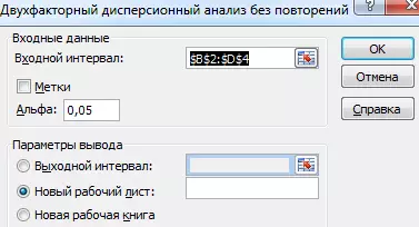
Dispersion analysis is carried out with several variables. Consider this on the example: you need to find out how quickly the reaction to the sound of different volumes in men and women is manifested.

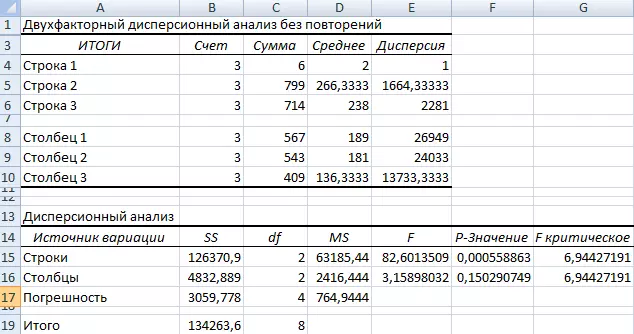
26.

1. Open an "data analysis", you need to find a two-factor dispersion analysis without repetitions.
2. Input interval - cells where data is contained (without a hat). We bring results to the new sheet and click "OK".

27.

The indicator F is larger than the F-critical - this means that the floor affects the reaction rate to the sound.

28.

Conclusion

This article described in detail the sensitivity analysis in the Excel table processor, so that each user can figure out the methods of its use.

Message The sensitivity analysis in Excel (sample data table) appeared first to information technology.